The input of the tool set is the negation of the LRTL behavioral model in Conjunctive Normal Form. This means that we should perform the first three steps of the algorithm manually. The first three steps are as below:

consider F= ¬(SP → SA);

convert it to a Presburger formula: F_Presb=Presb(F);

and, construct the Skolem formula:F_CNF Skolem(F).

We will be using the data from this SATS project to demonstrate how jLRTLV works.

Once we have our data in format that we like (through the first 3 steps of the LRTL algorithm, as explained here) we do the following things:

• Run extractdata.sh on the specification file with the negated SA. This creates a file with the literals, and a file with all the clauses, and a file with all the symbols.
• Run the jLRTLV application with the specification file as a parameter.

jLRTLV then performs the following steps:

1. Reads and parses literals.
2. Reads and parses symbols.
3. Reads and parses clauses.
4. Creates the column matrix B from the right side of all inequalities in the specification and it's negated safety assertion
5. Creates the coefficient matrix A.
6. Finds all subsystems in the system, if they exist.
7. Generates positive dependencies.
8. Attempts to find a generic lambda for the entire system if it is a system for which this is a valid operation.
9. Generates negative dependencies, if they exist.
10. Attempts Solves the system using SAT4J.

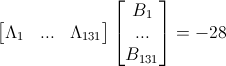
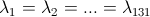
For this set of input data, the generic solution [ a a ... a ] is obtained for row vector Λ_1x131 =[ λ₁ ... λ₁₃₁ ] by solving Λ_1x131A_131x76=0. Positive row vectors Λ_1x131=[ a a ... a] are identified such that a=1. Therefore, ΛB=-28a<0 can be held by replacing the variable a with any positive number. As the negative linear dependent of the system exists, the negative clause {¬A₁,¬A₂,...,¬A₁₃₁} can be added to the set of negative clauses F_neg. Regarding the LRTL algorithm, the negative clause F_neg must be united with F_pos to build the propositional formula PF= F_pos∪F_neg. The unsatisfiability of the PF, which is the negation of SP→SA, requires that SP→SA is a theorem; the specification of the system implies its safety assertions.

The following matrix is the matrix that is created upon the processing of the SATS data in text format: SATS csv. This matrix has been debugged and has columns which all sum to zero. Because of this we know that the if sum of the right side of all inequalities in the system is negative then there is a generic positive lambda which produces a negative scalar value when multiplied by the column vector consisting of the right side of all inequalities in the specification. In this specific scenario this is our expected ( and actual ) result:

We have a lambda consisting of all equal values.